Counting by many groups — sometimes referred to as crosstab reviews — can be a beneficial way to seem at details ranging from community feeling surveys to health care assessments. For instance, how did men and women vote by gender and age team? How quite a few software package developers who use both R and Python are males vs. ladies?
There are a great deal of approaches to do this type of counting by groups in R. In this article, I’d like to share some of my favorites.
For the demos in this report, I’ll use a subset of the Stack Overflow Developers survey, which surveys developers on dozens of topics ranging from salaries to systems utilized. I’ll whittle it down with columns for languages utilized, gender, and if they code as a passion. I also added my personal LanguageGroup column for whether a developer described using R, Python, both, or neither.
If you’d like to follow together, the previous page of this report has guidelines on how to download and wrangle the details to get the identical details set I’m using.
The details has 1 row for each survey response, and the 4 columns are all characters.
str(mydata)
'data.frame':83379 obs. of  four variables:
 $ Gender            : chr  "Person" "Person" "Person" "Person" ...
 $ LanguageWorkedWith: chr  "HTML/CSSJavaJavaScriptPython" "C++HTML/CSSPython" "HTML/CSS" "CC++C#PythonSQL" ...
 $ Hobbyist          : chr  "Certainly" "No" "Certainly" "No" ...
 $ LanguageGroup     : chr  "Python" "Python" "Neither" "Python" ...
I filtered the raw details to make the crosstabs much more workable, together with eliminating missing values and using the two major genders only, Person and Female.
The janitor bundle
So, what is the gender breakdown within just each language team? For this form of reporting in a details body, 1 of my go-to resources is the janitor package’s tabyl() purpose.
The standard tabyl() purpose returns a details body with counts. The initially column title you add to a tabyl() argument turns into the row, and the second 1 the column.
library(janitor)
tabyl(mydata, Gender, LanguageGroup)
Gender Each Neither Python   R
    Person 3264   43908  29044 969
  Female  374    3705   1940 one hundred seventy five
What is good about tabyl() is it is incredibly uncomplicated to produce percents, much too. If you want to see percents for each column as an alternative of raw totals, add adorn_percentages("col"). You can then pipe these success into a formatting purpose these as adorn_pct_formatting().
tabyl(mydata, Gender, LanguageGroup) {fb741301fcc9e6a089210a2d6dd4da375f6d1577f4d7524c5633222b81dec1ca}>{fb741301fcc9e6a089210a2d6dd4da375f6d1577f4d7524c5633222b81dec1ca}
adorn_percentages("col") {fb741301fcc9e6a089210a2d6dd4da375f6d1577f4d7524c5633222b81dec1ca}>{fb741301fcc9e6a089210a2d6dd4da375f6d1577f4d7524c5633222b81dec1ca}
adorn_pct_formatting(digits = one)Gender  Each Neither Python     R
    Person 89.seven{fb741301fcc9e6a089210a2d6dd4da375f6d1577f4d7524c5633222b81dec1ca}   ninety two.2{fb741301fcc9e6a089210a2d6dd4da375f6d1577f4d7524c5633222b81dec1ca}  93.seven{fb741301fcc9e6a089210a2d6dd4da375f6d1577f4d7524c5633222b81dec1ca} eighty four.seven{fb741301fcc9e6a089210a2d6dd4da375f6d1577f4d7524c5633222b81dec1ca}
  Female 10.3{fb741301fcc9e6a089210a2d6dd4da375f6d1577f4d7524c5633222b81dec1ca}    seven.8{fb741301fcc9e6a089210a2d6dd4da375f6d1577f4d7524c5633222b81dec1ca}   6.3{fb741301fcc9e6a089210a2d6dd4da375f6d1577f4d7524c5633222b81dec1ca} 15.3{fb741301fcc9e6a089210a2d6dd4da375f6d1577f4d7524c5633222b81dec1ca}
To see percents by row, add adorn_percentages("row").
If you want to add a 3rd variable, these as Hobbyist, that’s uncomplicated much too.
tabyl(mydata, Gender, LanguageGroup, Hobbyist) {fb741301fcc9e6a089210a2d6dd4da375f6d1577f4d7524c5633222b81dec1ca}>{fb741301fcc9e6a089210a2d6dd4da375f6d1577f4d7524c5633222b81dec1ca}
adorn_percentages("col") {fb741301fcc9e6a089210a2d6dd4da375f6d1577f4d7524c5633222b81dec1ca}>{fb741301fcc9e6a089210a2d6dd4da375f6d1577f4d7524c5633222b81dec1ca}
adorn_pct_formatting(digits = one)
On the other hand, it will get a little more durable to visually examine success in much more than two stages this way. This code returns a record with 1 details body for each 3rd-level choice:
$No
 Gender  Each Neither Python     R
    Person 79.6{fb741301fcc9e6a089210a2d6dd4da375f6d1577f4d7524c5633222b81dec1ca}   86.seven{fb741301fcc9e6a089210a2d6dd4da375f6d1577f4d7524c5633222b81dec1ca}  86.four{fb741301fcc9e6a089210a2d6dd4da375f6d1577f4d7524c5633222b81dec1ca} seventy four.6{fb741301fcc9e6a089210a2d6dd4da375f6d1577f4d7524c5633222b81dec1ca}
  Female twenty.four{fb741301fcc9e6a089210a2d6dd4da375f6d1577f4d7524c5633222b81dec1ca}   thirteen.3{fb741301fcc9e6a089210a2d6dd4da375f6d1577f4d7524c5633222b81dec1ca}  thirteen.6{fb741301fcc9e6a089210a2d6dd4da375f6d1577f4d7524c5633222b81dec1ca} twenty five.four{fb741301fcc9e6a089210a2d6dd4da375f6d1577f4d7524c5633222b81dec1ca}

$Certainly
 Gender  Each Neither Python     R
    Person ninety one.6{fb741301fcc9e6a089210a2d6dd4da375f6d1577f4d7524c5633222b81dec1ca}   93.9{fb741301fcc9e6a089210a2d6dd4da375f6d1577f4d7524c5633222b81dec1ca}  95.{fb741301fcc9e6a089210a2d6dd4da375f6d1577f4d7524c5633222b81dec1ca} 88.{fb741301fcc9e6a089210a2d6dd4da375f6d1577f4d7524c5633222b81dec1ca}
  Female  8.four{fb741301fcc9e6a089210a2d6dd4da375f6d1577f4d7524c5633222b81dec1ca}    6.one{fb741301fcc9e6a089210a2d6dd4da375f6d1577f4d7524c5633222b81dec1ca}   5.{fb741301fcc9e6a089210a2d6dd4da375f6d1577f4d7524c5633222b81dec1ca} twelve.{fb741301fcc9e6a089210a2d6dd4da375f6d1577f4d7524c5633222b81dec1ca}
The CGPfunctions bundle
The CGPfunctions bundle is worthy of a seem for some fast and uncomplicated approaches to visualize crosstab details. Install it from CRAN with the standard set up.packages("CGPfunctions").
The bundle has two functions of fascination for analyzing crosstabs: PlotXTabs() and PlotXTabs2(). This code returns bar graphs of the details (initially graph beneath):
library(CGPfunctions)
PlotXTabs(mydata)
 Display screen shot by Sharon Machlis, IDG
Consequence of PlotXTabs(mydata).
PlotXTabs2(mydata) creates a graph with a various seem, and some statistical summaries (second graph at still left).
If you really do not will need or want these summaries, you can eliminate them with success.subtitle = False, these as PlotXTabs2(mydata, LanguageGroup, Gender, success.subtitle = False).
 Display screen shot by Sharon Machlis, IDG
Consequence of PlotXTabs(mydata).
PlotXTabs2() has a few of dozen argument choices, together with title, caption, legends, shade plan, and 1 of 4 plot forms: aspect, stack, mosaic, or percent. There are also choices familiar to ggplot2 people, these as ggtheme and palette. You can see much more particulars in the function’s enable file.
The vtree bundle
The vtree bundle generates graphics for crosstabs as opposed to graphs. Running the principal vtree() purpose on 1 variable, these as
library(vtree)
vtree(mydata, "LanguageGroup")
will get you this standard response:
 Sharon Machlis, IDG
Standard vtree() purpose on 1 variable.
I’m not eager on the shade defaults listed here, but you can swap in an RColorBrewer palette. vtree’s palette argument uses palette quantities, not names you can see how they’re numbered in the vtree bundle documentation. I could opt for 3 for Greens and 5 for Purples, for instance. However, these defaults give you a much more extreme shade for decrease count quantities, which does not always make sense (and does not operate perfectly for me in this instance). I can modify that default behavior with sortfill = Real to use the much more extreme shade for the increased benefit.
vtree(mydata, "LanguageGroup", palette = 3, sortfill = Real)
 Sharon Machlis, IDG
vtree() after altering to a new palette.
If you come across the darkish shade helps make it challenging to browse textual content, there are some choices. A single alternative is to use the plain argument, these as vtree(mydata, "LanguageGroup", plain = Real). Another alternative is to set a solitary fill color instead of a palette, using the fillcolor argument, these as vtree(mydata, LanguageGroup", fillcolor = "#99d8c9").
To seem at two variables in a crosstab report, simply just add a second column title and palette or shade if you really do not want the default. You can use the plain alternative or specify two palettes or two hues. Down below I selected unique hues as an alternative of palettes, and I also rotated the graph to browse vertically.
vtree(mydata, c("LanguageGroup", "Gender"),
fillcolor = c( LanguageGroup = "#e7d4e8", Gender = "#99d8c9"),
horiz = False)
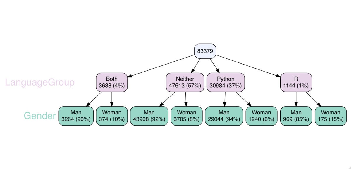 Sharon Machlis, IDG
vtree() for two variables.
You can add much more than two groups, although it will get a little bit more durable to browse and follow as the tree grows. If you are only interested in some of the branches, you can specify which to show with the hold argument. Down below, I set vtree() to show only men and women who use R without having Python or who use both R and Python.
vtree(mydata, c("Gender", "LanguageGroup", "Hobbyist"),
horiz = False, fillcolor = c(LanguageGroup = "#e7d4e8",
Gender = "#99d8c9", Hobbyist = "#9ecae1"),
hold = record(LanguageGroup = c("R", "Each")), showcount = False)
With the tree getting so active, I think it allows to have possibly the count or the percent as node labels, not both. So that previous argument in the code earlier mentioned, showcount = False, sets the graph to show only percents and not counts.
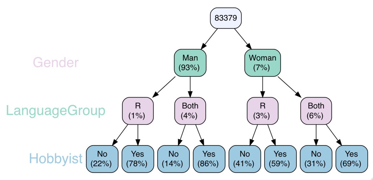 Sharon Machlis, IDG
Three-level vtree graphic with a subset of nodes, displaying percents only.
A lot more count by team choices
There are other beneficial approaches to team and count in R, together with foundation R, dplyr, and details.desk. Foundation R has the xtabs() purpose precisely for this task. Take note the system syntax beneath: a tilde and then 1 variable additionally a different variable.
xtabs(~ LanguageGroup + Gender, details = mydata)
Gender
LanguageGroup   Person Female
      Each     3264   374
      Neither 43908  3705
      Python  29044  1940
      R         969   one hundred seventy five
dplyr’s count() purpose combines “group by” and “count rows in each group” into a solitary purpose.
library(dplyr)
my_summary <- mydata {fb741301fcc9e6a089210a2d6dd4da375f6d1577f4d7524c5633222b81dec1ca}>{fb741301fcc9e6a089210a2d6dd4da375f6d1577f4d7524c5633222b81dec1ca}
count(LanguageGroup, Gender, Hobbyist, form = Real)my_summary LanguageGroup Gender Hobbyist n one Neither Person Certainly 34419 2 Python Person Certainly 25093 3 Neither Person No 9489 four Python Person No 3951 5 Each Person Certainly 2807 6 Neither Female Certainly 2250 seven Neither Female No 1455 8 Python Female Certainly 1317 9 R Person Certainly 757 10 Python Female No 623 eleven Each Person No 457 twelve Each Female Certainly 257 thirteen R Person No 212 fourteen Each Female No 117 15 R Female Certainly 103 16 R Female No 72
In the 3 lines of code beneath, I load the details.desk bundle, make a details.desk from my details, and then use the particular .N details.desk image that stands for variety of rows in a team.
library(details.desk)
mydt <- setDT(mydata)
mydt[, .N, by = .(LanguageGroup, Gender, Hobbyist)]
Visualizing with ggplot2
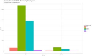
As with most details, ggplot2 is a good choice to visualize summarized success. The initially ggplot graph beneath plots LanguageGroup on the X axis and the count for each on the Y axis. Fill shade signifies whether someone claims they code as a passion. And, facet_wrap claims: Make a independent graph for each benefit in the Gender column.
library(ggplot2)
ggplot(my_summary, aes(LanguageGroup, n, fill = Hobbyist)) +
geom_bar(stat = "id") +
facet_wrap(sides = vars(Gender))
 Sharon Machlis, IDG
Making use of ggplot2 to examine language use by gender.
Due to the fact there are rather few ladies in the sample, it is tricky to examine percentages across genders when both graphs use the identical Y-axis scale. I can modify that, nevertheless, so each graph uses a independent scale, by including the argument scales = “free_y” to the facet_wrap() purpose:
ggplot(my_summary, aes(LanguageGroup, n, fill = Hobbyist)) +
geom_bar(stat = "id") +
facet_wrap(sides = vars(Gender), scales = "cost-free_y")
Now it is a lot easier to examine many variables by gender.
For much more R guidelines, head to the “Do A lot more With R” page on InfoWorld or check out out the “Do A lot more With R” YouTube playlist.
See the subsequent page for facts on how to download and wrangle details utilized in this demo.